The Complete Codes

Fractional Knapsack Problem A thief has a bag or knapsack that can contain the maximum weight W of his loot. There are n items and the weight of an ith item is wi and it worth vi. Any amount of item can be put into the bag i.e. xi fraction of item can be collected, where 0<=xi<=1. Here the objective is to collect the items that maximize the total profit earned. Here we arrange the items by ratio vi/wi. Algorithm GreedyFracKnapsack (W, n) {     for (i = 1 ; i <= n; i++)     {         x [i] = 0.0 ;     }     tempW = W;     for (i = 1 ; i <= n; i++)     {         if ( w [i] > tempW)             then break ;         x [i] = 1.0 ;         tempW -= w [i];     }     if (i <= n)         x [i] = tempW / w [i]; } We can see that the above algorithm just contains a single loop i.e. no nested loops the running time for the above algorithm is O(n). However our requirement is that v[1 ... n] and w[1 ... n] are sorted, so we can use the sorting method to sort it in O(n log n

  NP-Completeness Most of the problems considered up to now can be solved by algorithms in worst-case polynomial time. There are many problems and it is not necessary that all the problems have an apparent solution. This concept, somehow, can be applied to solving the problem using computers. The computer can solve: some problems in a limited time e.g. sorting, some problems require an unmanageable amount of time e.g. Hamiltonian cycles, and some problems cannot be solved e.g. I-lasting Problem. In this section, we concentrate on the specific class of problems called NP-complete problems (will be defined later). Tractable and Intractable Problems We call problems as tractable or easy if the problem can be solved using polynomial-time algorithms. The problems that cannot be solved in polynomial time but require a super polynomial-time algorithm are called intractable or hard problems. There are many problems for which no algorithm with running time better than exponential time is kn

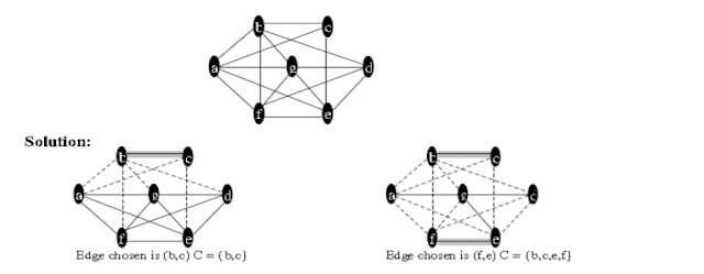
Approximation Algorithms An approximate algorithm is a way of dealing with NP—completeness for optimization problem. This technique does not guarantee the best solution. The goal of an approximation algorithm is to come as close as possible to the optimum value in a reasonable amount of time which is at most polynomial time. If we are dealing with optimization problem {maximization or minimization} with feasible solution having positive cost then it is worthy to look at approximate algorithm for near optimal solution. Vertex Cover Problem A vertex cover of an undirected graph G =(V.E) is a subset V‘ I V such that for all edges (u.v) EE either usV’ or vsV’ or u and v 2 V’. The problem here is to find the vertex cover of minimum size in a given graph G. Optimal vertex—cover is the optimization version of an NP—complete problem but it is not too hard to find a vertex-cover that is near optimal. Algorithm ApproxVertexCover {G} { C ={ } ; E’ = E while E' is not empty do

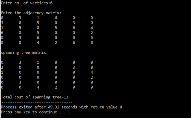
C Program For Prim's Algorithm To Find Shortest Path #include <stdio.h> #include <stdlib.h> #define infinity 9999 #define MAX 20 int G [ MAX ][ MAX ], spanning [ MAX ][ MAX ], n ; int prims (); int main () {     int i , j , total_cost ;     printf ( "Enter no. of vertices:" );     scanf ( " %d " , & n );     printf ( " \n Enter the adjacency matrix: \n " );     for ( i = 0 ; i < n ; i ++)         for ( j = 0 ; j < n ; j ++)             scanf ( " %d " , & G [ i ][ j ]);     total_cost = prims ();     printf ( " \n spanning tree matrix: \n " );     for ( i = 0 ; i < n ; i ++)     {         printf ( " \n " );         for ( j = 0 ; j < n ; j ++)             printf ( " %d \t " , spanning [ i ][ j ]);     }     printf ( " \n\n Total cost of spanning tree= %d " , total_cost );     return 0 ; } int prims () {     int cost [ MAX ][ MAX ];     int u ,

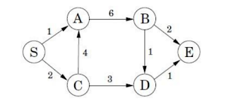
Directed Acyclic Graph (DAG) DAG, here directed means that each edge has an arrow denoting that the edge can be traversed in only that particular direction. Acyclic means that the graph has no cycles, i.e., starting at one node, you can never end up at the same node. DAG can be used to find the shortest path from a given source node to all other nodes. To find the shortest path by using DAG, first of all sort the vertices of the graph topologically and then relax the vertices in topological order.

Prim’s Algorithm This is another algorithm for finding MST. The idea behind this algorithm is just take any arbitrary vertex and choose the edge with minimum weight incident on the chosen vertex. Add the vertex and continue the above process taking all the vertices added. Remember the cycle must be avoided. Algorithm: PrimMST(G) { T = ?; // T is a set of edges of MST S = {s} ; //s is randomly chosen vertex and S is set of vertices while(S != V) { e = (u,v) an edge of minimum weight incident to vertices in T and not forming a simple circuit in T if added to T i.e. u ??S and v??V-S T = T ??{(u,v)}; S = S ??{v}; } } Analysis: In the above algorithm while loop execute O(V). The edge of minimum weight incident on a vertex can be found in O(E), so the total time is O(EV). We can improve the performance of the above algorithm by choosing better data structures as priority queue and normally it will be seen that the running time of prim’s algorithm is O(ElogV)!.

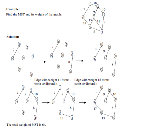
Minimum Spanning Tree Given an undirected graph G = (V,E), a subgraph T =(V,E’) of G is a spanning tree if and only if T is a tree. The MST is a spanning tree of a connected weighted graph such that the total sum of the weights of all edges eÎE’ is minimum amongst all the sum of edges that would give a spanning tree.

Graph Traversals There are a number of approaches used for solving problems on graphs. One of the most important approaches is based on the notion of systematically visiting all the vertices and edges of a graph. The reason for this is that these traversals impose a type of tree structure (or generally a forest) on the graph, and trees are usually much easier to reason about than general graphs. Depth First Search This is another technique that can be used to search the graph. Choose a vertex as a root and form a path by starting at a root vertex by successively adding vertices and edges. This process is continued until no possible path can be formed. If the path contains all the vertices then the tree consisting of this path is the DFS tree. Otherwise, we must add other edges and vertices. For this move back from the last vertex that is met in the previous path and find whether it is possible to find a new path starting from the vertex just met. If there is such a path

Graph Traversals There are a number of approaches used for solving problems on graphs. One of the most important approaches is based on the notion of systematically visiting all the vertices and edges of a graph. The reason for this is that these traversals impose a type of tree structure (or generally a forest) on the graph, and trees are usually much easier to reason about than general graphs. Breadth-first search This is one of the simplest methods of graph searching. Choose some vertex arbitrarily as a root. Add all the vertices and edges that are incident in the root. The new vertices added will become the vertices at level 1 of the BFS tree. Form the set of the added vertices of level 1, and find other vertices, such that they are connected by edges at level 1 vertices. Follow the above step until all the vertices are added. Algorithm: BFS ( G , s ) // s is start vertex {     T = {s};     L = Φ; // an empty queue     Enqueue (L, s );     while (L != Φ)     {  

Job Sequencing with Deadline We are given a set of n jobs. Associated with each job I, di>=0 is an integer deadline and pi>=O is profit. For any job i profit is earned if the job is completed by the deadline. To complete a job one has to process a job for one unit of time. Our aim is to find a feasible subset of jobs such that profit is maximum. Example n=4, (p1,p2,p3,p4)=(100,10,15,27),(d1,d2,d3,d4)=(2,1,2,1) n=4, (p1,p4,p3,p2)=(100,27,15,10),(d1,d4,d3,d2)=(2,1,2,1) We have to try all the possibilities, complexity is O(n!). Greedy strategy using total profit as optimization function to above example. Begin with J= Job 1 considered, and added to J ->J={1} Job 4 considered, and added to J -> J={1,4} Job 3 considered, but discarded because not feasible   ->J={1,4} Job 2 considered, but discarded because not feasible   -> J={1,4} The final solution is J={1,4} with a total profit of 127 and it is optimal Algorithm: Assume

Huffman coding Huffman coding is an algorithm for the lossless compression of files based on the frequency of occurrence of a symbol in the file that is being compressed. In any file, certain characters are used more than others. Using binary representation, the number of bits required to represent each character depends upon the number of characters that have to be represented. Using one bit we can represent two characters, i.e., 0 represents the first character and l represents the second character. Using two bits we can represent four characters, and so on. Unlike ASCII code, which is a fixed-length code using seven bits per character, Huffman compression is a variable-length coding system that assigns smaller codes for more frequently used characters and larger codes for less frequently used characters in order to reduce the size of files being compressed and transferred. For example, in a file with the following data: ‘XXXXXXYYYYZZ. The frequency of "X" is 6, t

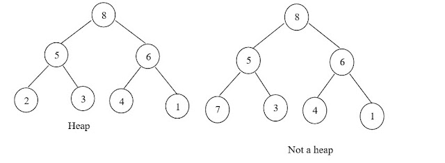
Heap Sort   A heap is a nearly complete binary tree with the following two properties: Structural property: all levels are full, except possibly the last one, which is filled from left to right Order (heap) property: for any node x, Parent(x) ≥ x Array Representation of Heaps A heap can be stored as an array A. Root of tree is A[1] Left child of A[i] = A[2i] Right child of A[i] = A[2i + 1] Parent of A[i] = A[ i/2 ] Heapsize[A] ≤ length[A] The elements in the subarray A[( ⌊ n/2 ⌋ +1) .. n] are leaves Max-heaps (largest element at root), have the max-heap property:   for all nodes i, excluding the root:     A[PARENT(i)] ≥ A[i] Min-heaps (smallest element at root), have the min-heap property: for all nodes i, excluding the root:   A[PARENT(i)] ≤ A[i] Adding/Deleting Nodes New nodes are always inserted at the bottom level (left to right) and nodes are removed from the bottom level (right to left). Operations on Heaps Maintai

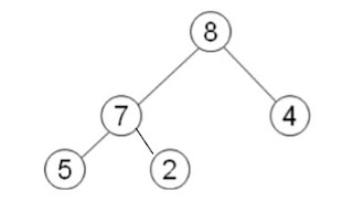
Heap A heap is a complete tree with an ordering-relation R holding between each node and its descendant. Note that the complete tree here means tree can miss only rightmost part of the bottom level. R can be smaller-than, bigger-than. E.g. Heap with degree 2 and R is “bigger than”. Heap Sort  Build a heap from the given set (O(n)) time, then repeatedly remove the elements from the heap (O(n log n)). Implementation Heaps are implemented by using arrays. Insertion and deletion of an element takes O(log n) time. More on this later Heap Sort Pseudo Code Heapsort ( A ) {     BuildHeap ( A )     for i <- length (A) downto 2 {       exchange A [ 1 ] <-> A [i]       heapsize <- heapsize - 1       Heapify (A, 1 ) } BuildHeap (A)    {    heapsize <- length (A)     for i <- floor ( length/ 2 ) downto 1       Heapify (A, i)    }     Heapify (A, i)    {        le < - left (i)                    ri < - right (i)                             if (le